


Jupyter Notebooks are a powerful open-source tool that allows users to create and share documents that contain live code, equations, visualizations, and narrative text. They are widely used in data science, machine learning, and scientific computing for interactive coding and data analysis. This tutorial will guide you through installing Jupyter, using basic features, and performing data analysis interactively.
1. Installing Jupyter Notebook
To start using Jupyter Notebooks, you need to install it. You can install Jupyter via Anaconda (recommended for beginners) or pip (for advanced users).
Using Anaconda
Anaconda is a popular Python distribution that comes with Jupyter Notebook pre-installed.
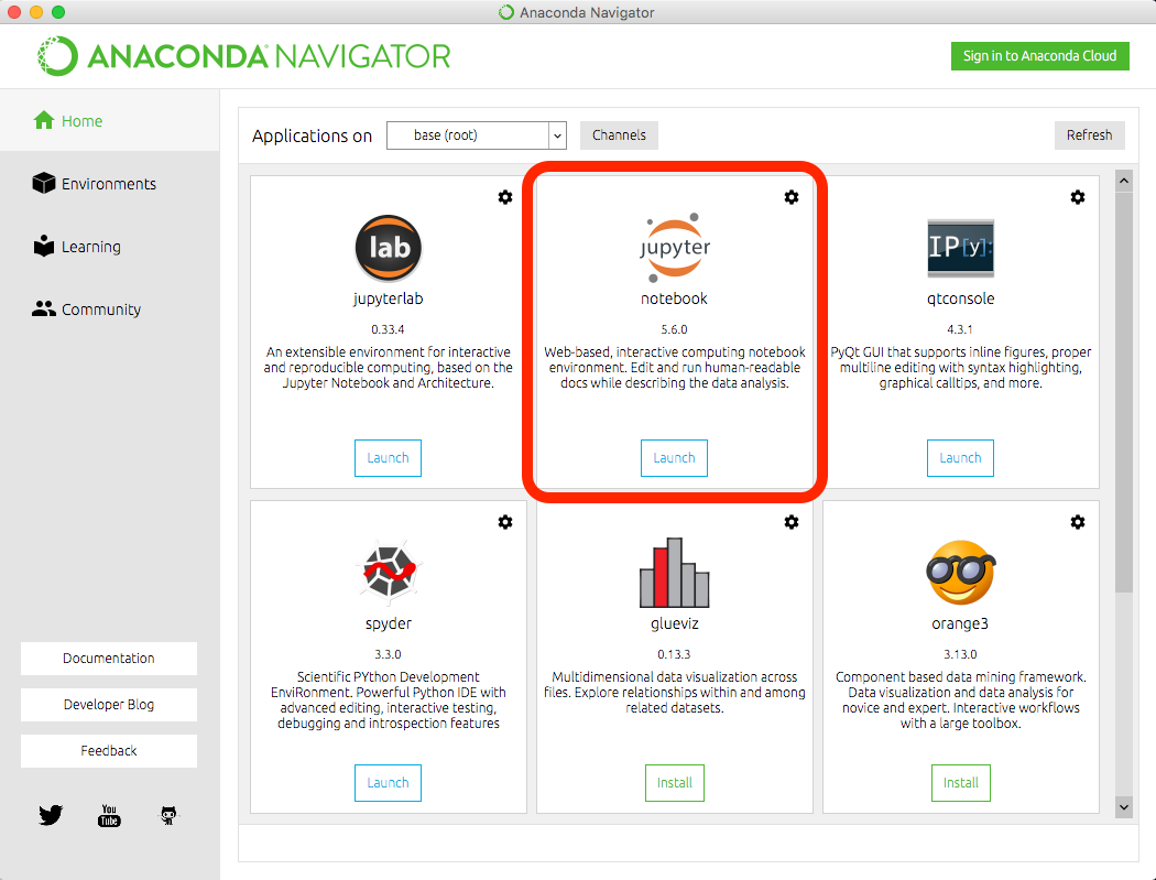
- Download and install Anaconda
- Open Anaconda Navigator and launch Jupyter Notebook
- You should see a dashboard like the one below:
Using pip
If you already have Python installed, you can install Jupyter Notebook using pip:

Once installed, launch Jupyter Notebook with:

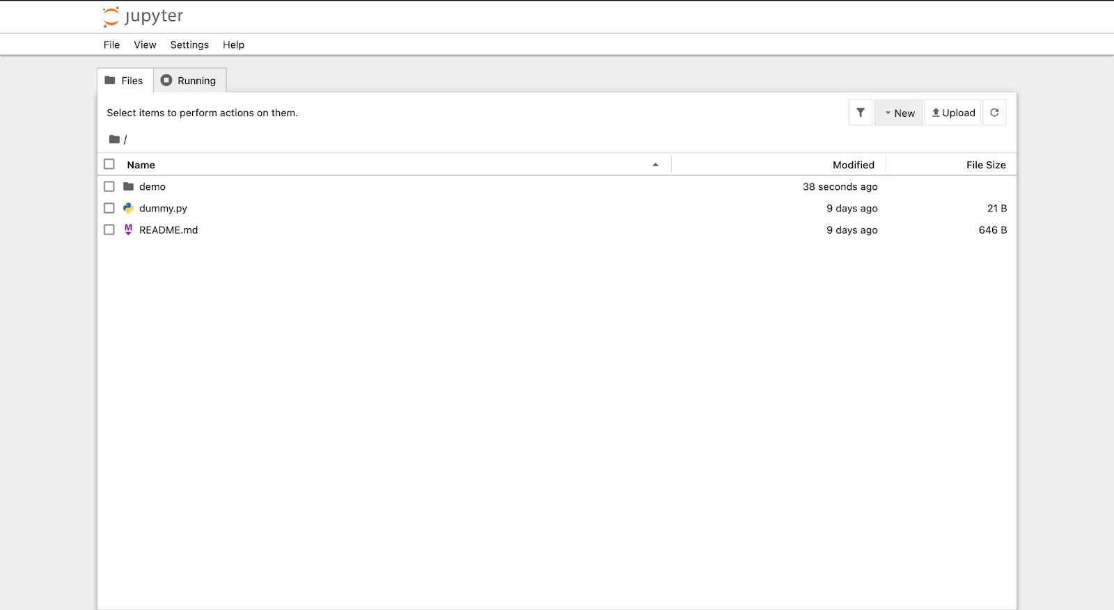
2. Navigating the Jupyter Interface
After launching Jupyter Notebook, you’ll see the Jupyter dashboard. It shows the current directory’s files and allows you to create and open notebooks.
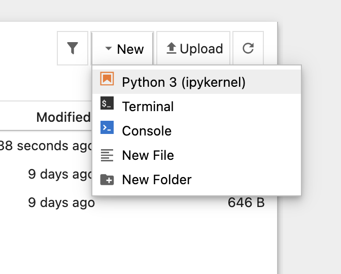
- Click New > Python 3 to create a new notebook.
- A new notebook consists of cells that can execute code or contain markdown for documentation.
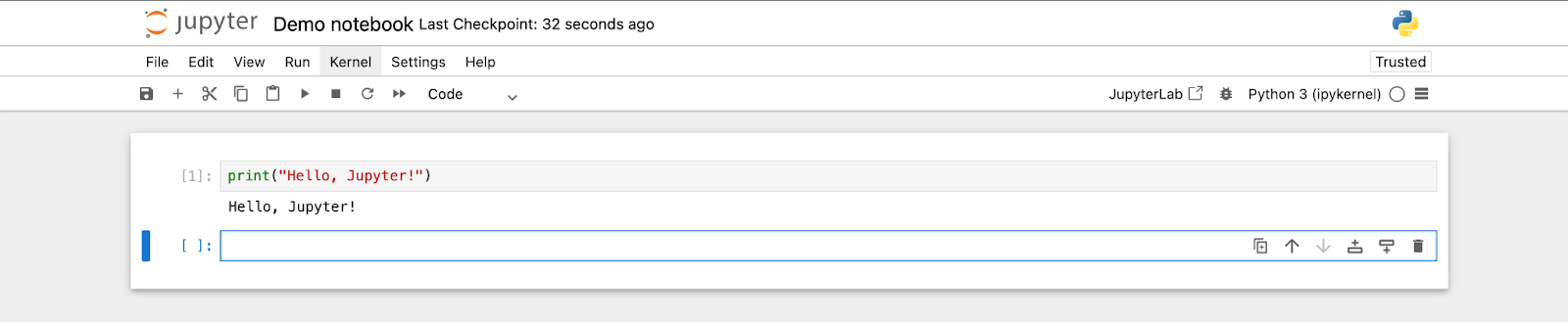
3. Running Code in Jupyter Notebook
Each notebook consists of cells that can hold code or markdown text.
Executing Python Code
To run a Python command inside a cell, type the code and press Shift + Enter.
Using Markdown Cells
You can switch a cell to Markdown (for formatted text) by selecting the cell and pressing Esc + M. Try adding headings, bullet points, or even LaTeX equations:


4. Importing and Visualizing Data
Jupyter is commonly used for data analysis. Let’s see how to load and visualize a dataset using Pandas and Matplotlib.
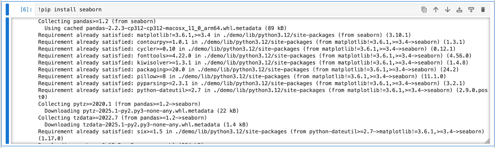
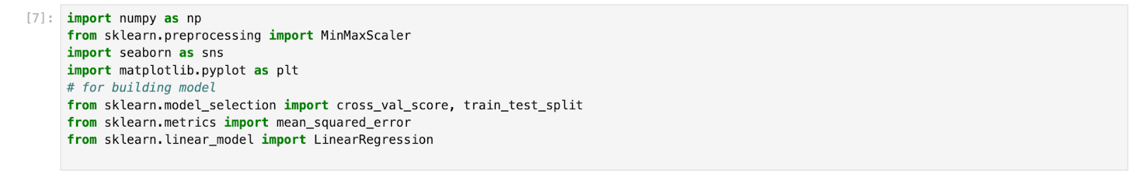
Importing Libraries
- seaborn: To install the seaborn python library you can write the below command in your jupyter notebook:
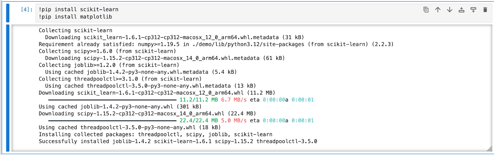
- matplotlib: To install the matplotlib and scikit-learn python library you can write the below command in your jupyter notebook:
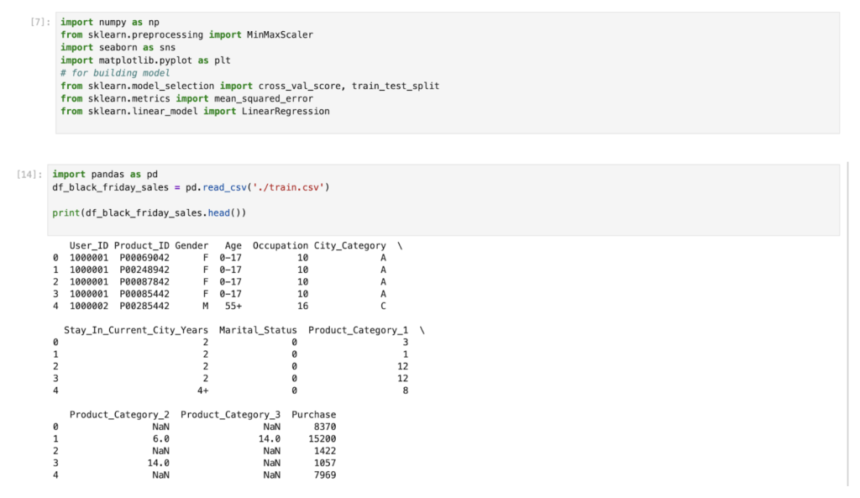
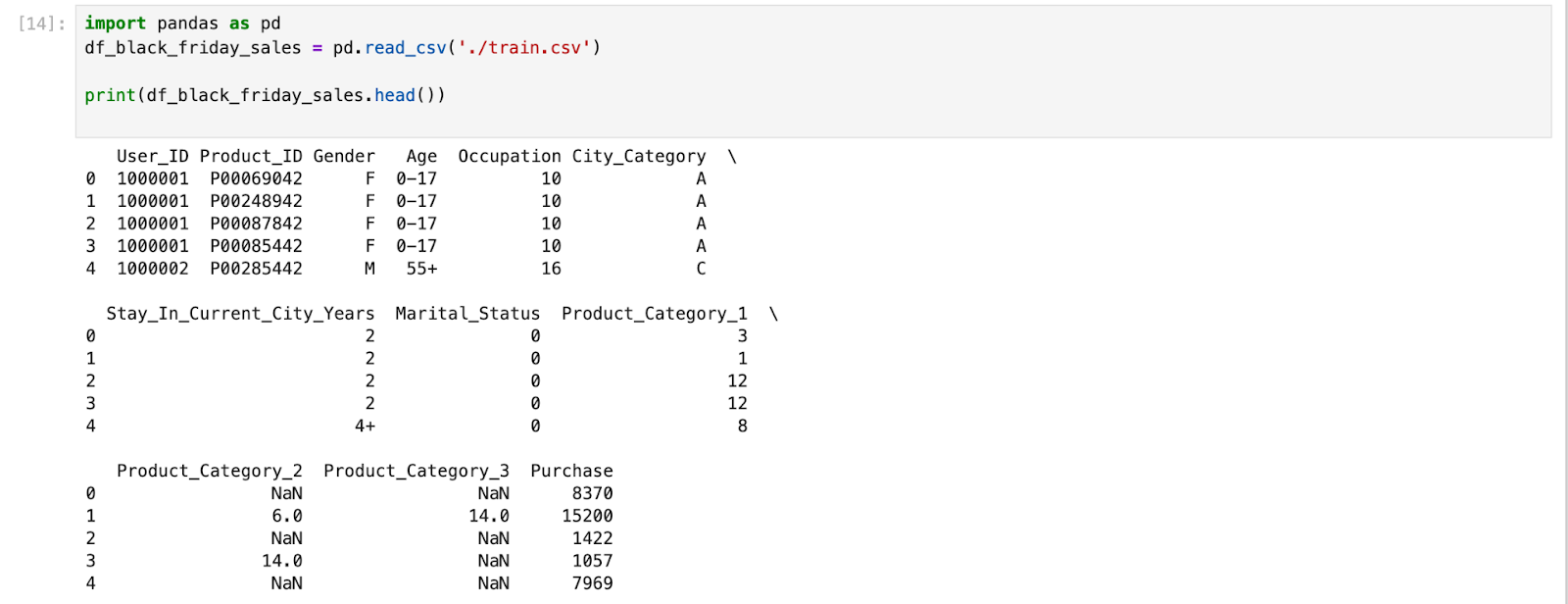
Loading a Dataset
There are many ways to import/load a dataset, either you can download a dataset or you can directly import it using Python library such as Seaborn, Scikit-learn (sklearn), NLTK, etc. The datasets that used here is a Black Friday Sales dataset from Kaggle.
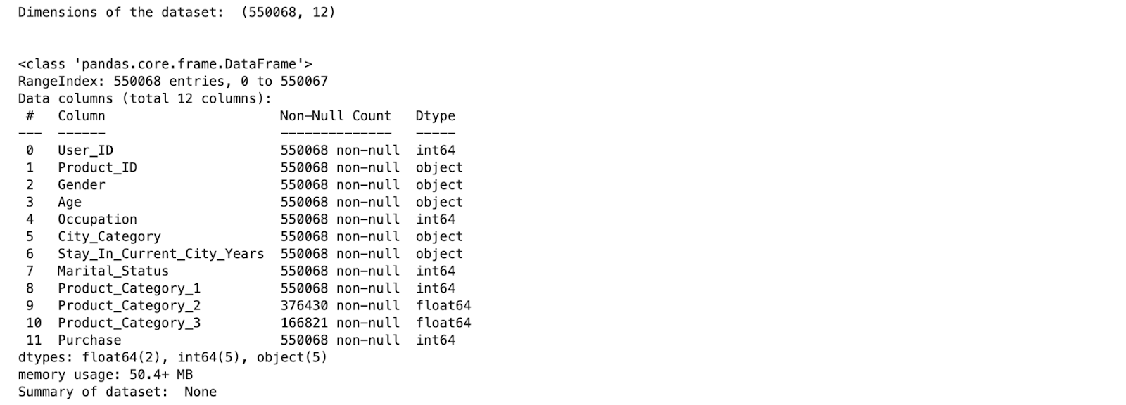
5. Data Analysis and Visualization
It is also an important step as it gives the distribution of the dataset and helps in finding similarities among features. Let’s start by looking at the shape of our dataset and concise summary of our dataset, using the below code:

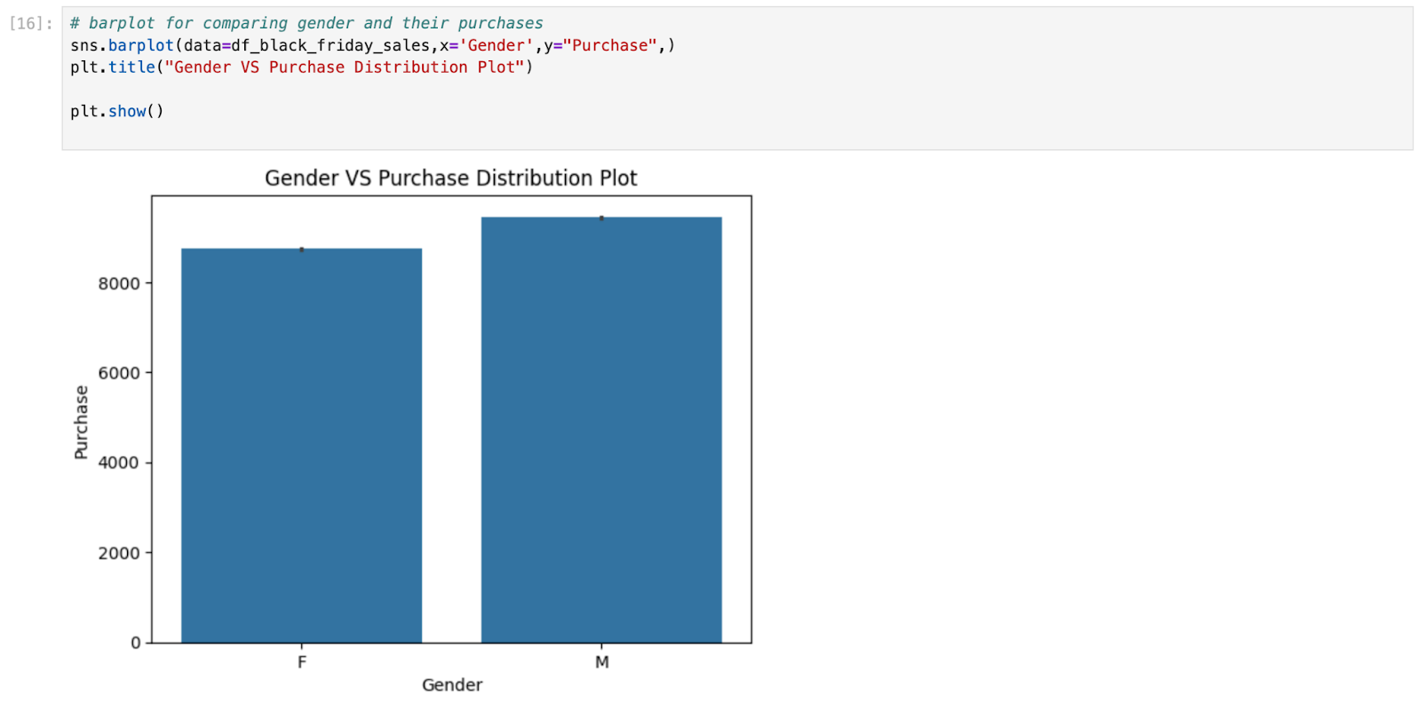
Data Visualization
Large and complex datasets are very difficult to understand but they can be easily understood with the help of graphs. Graphs/Plots can help in determining relationships between different entities and helps in comparing variables/features. Data Visulaisation means presenting the large and complex data in the form of graphs so that they are easily understandable. Begin by creating a bar plot that compares the percentage ratio of tips given by each gender , along with that make another graph to compare the average tips given by individuals of each gender.
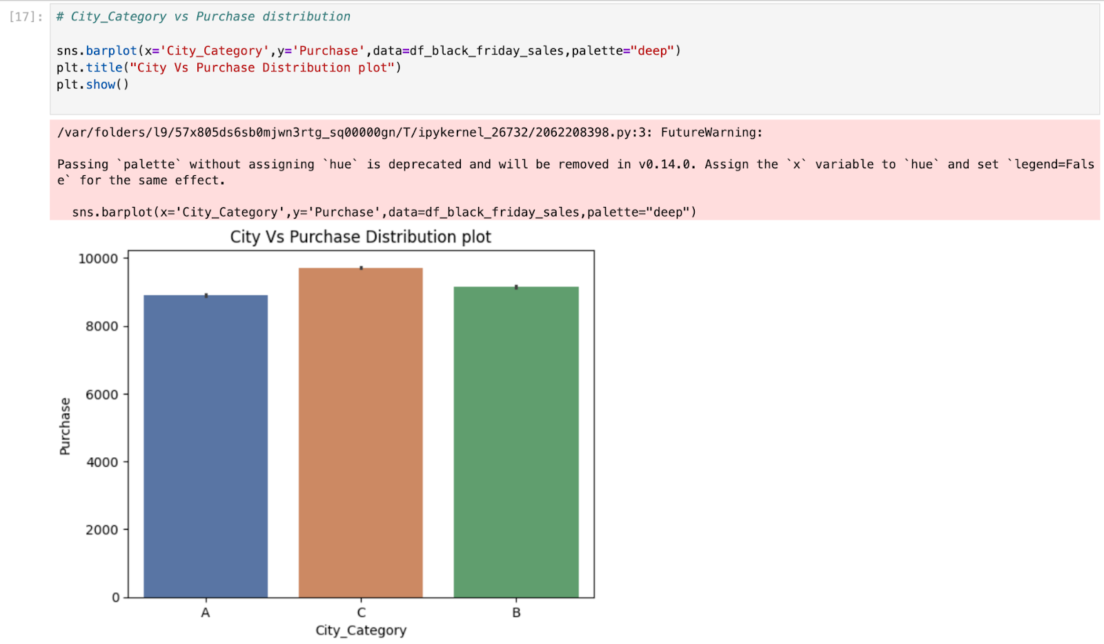
This code creates a bar plot using Seaborn to visualize the distribution of purchases (‘Purchase’) across different city categories (‘City_Category’) in the DataFrame ‘df_black_friday_sales’.
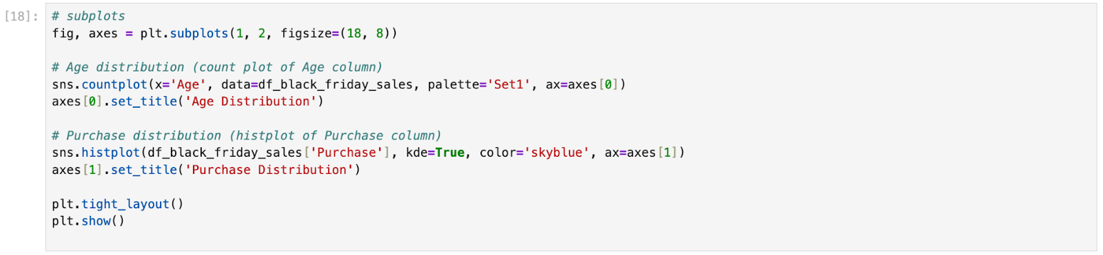
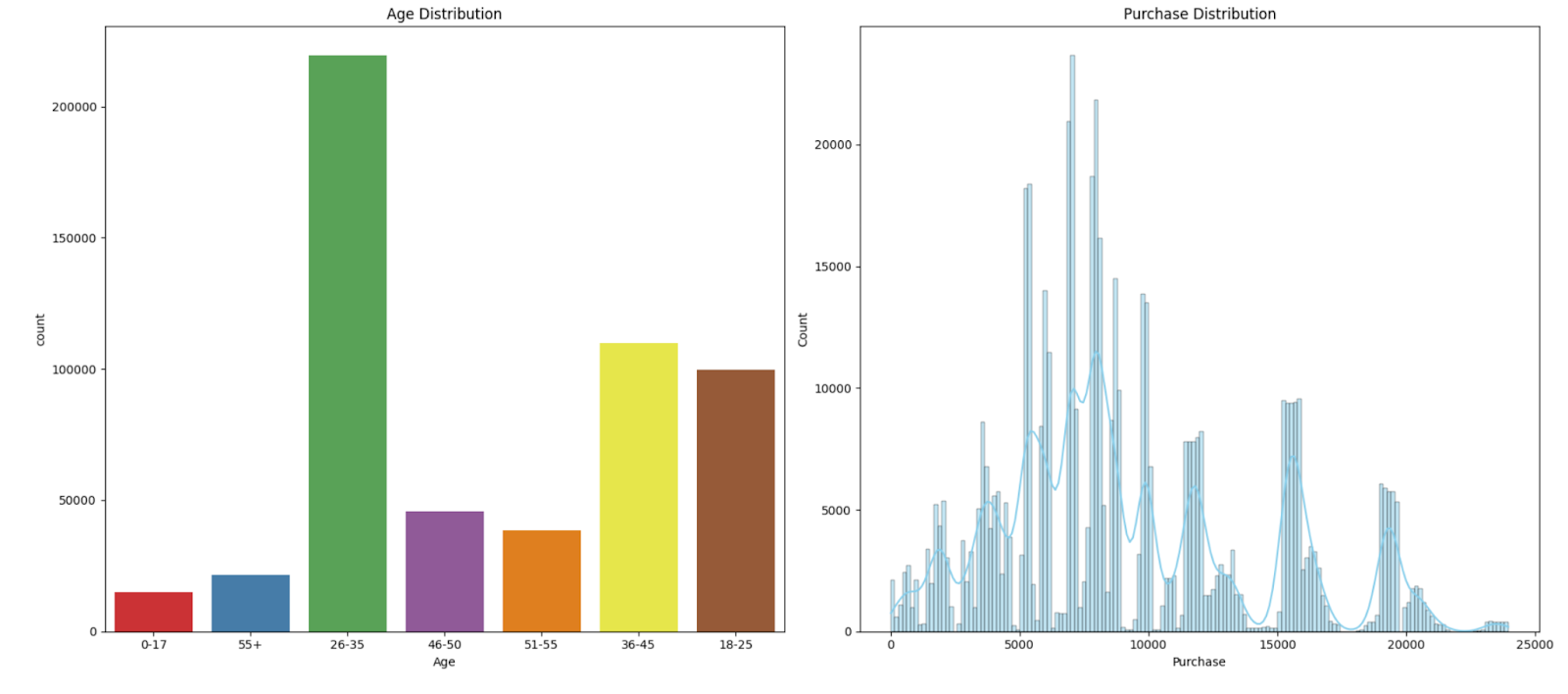
This code creates a figure with two subplots side by side. The first subplot displays a count plot of the ‘Age’ column from the ‘df_black_friday_sales’ DataFrame, while the second subplot shows a histogram and kernel density estimate (KDE) of the ‘Purchase’ column.
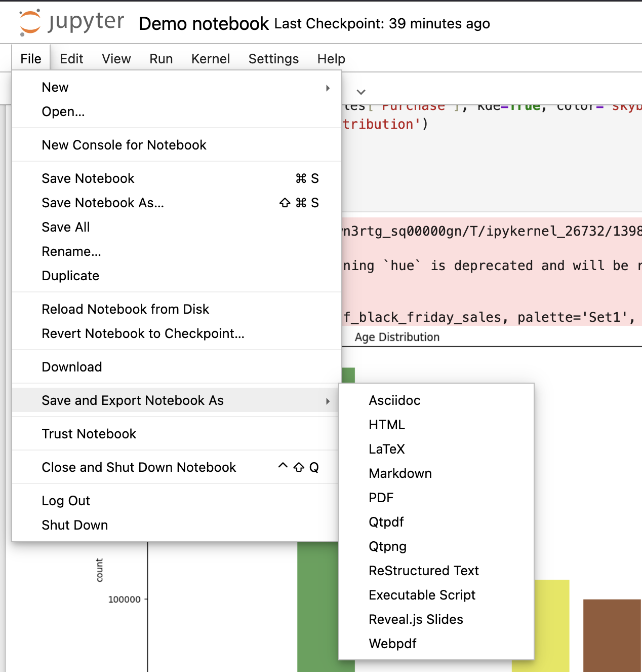
6. Saving and Exporting Notebooks
- Click File > Save and Export notebook as to save progress and export notebooks in various formats (PDF, HTML, Python script, etc.):
7. Best Practices
- Use markdown to document your work.
- Organize your notebook by using headings and sections.
- Use version control (e.g., GitHub) to track changes.
- Limit output size for large datasets.
Conclusion
This tutorial has covered the fundamental aspects of using Jupyter Notebooks for interactive coding and data analysis. We started with the installation process using both Anaconda and pip, followed by navigating the Jupyter interface. We then explored how to execute Python code, document work using Markdown, and perform data analysis using Pandas and visualization libraries like Matplotlib, scikit-learn and Seaborn.
By following the best practices outlined, you can create well-structured, reproducible, and efficient notebooks for your coding and data analysis projects. Now that you have a strong foundation, start experimenting with Jupyter Notebooks and explore its vast capabilities to enhance your workflow!
The post How to Use Jupyter Notebooks for Interactive Coding and Data Analysis appeared first on MarkTechPost.